

Background
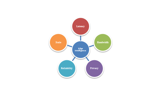
In recent years, deep learning-based Artificial Intelligence (AI) and Machine Learning (ML) models are moving from cloud to edge devices for various factors such as bandwidth, latency, etc as in Figure-1.
Power consumption, latency, hardware size are important aspects for inference at the edge. Moreover, The Models developed in the cloud using the GPUs are floating-point models.
Most importantly, it is highly desired for the edge inference hardware running Neural Networks do not have to support expensive Floating-Point units to suit the lower power and cost budgets. Compared to floating-point counterparts, the fixed point math engines are very area and power-efficient
Moreover, the model developed in the cloud needs to be quantized without significant loss of accuracy. An efficient quantization mechanism can quantize 32-bit Floating Point (FP) Models to 8-bit INT operations with a loss of accuracy of less than 0.5% for most of the models. This process reduces the memory footprint, compute requirements and thereby reduces the latency, and power required to do the inference of the models.
Most of the edge devices, including GPUs (who have FP arithmetic), now take advantage of lower precision and quantized operations. whereas, Quantization is a defacto step for edge inference. This blog talks about common methods for doing quantization, challenges, and methods to overcome them.
Types of Quantization
Primarily Three types of quantization techniques of neural networks listed in increasing order of complexity and accuracy.
- Power-2
- Symmetric
- Asymmetric
Power-2
Power-2 quantization uses only the left and right shifts of the data to perform the quantization. Shifts have a very low-cost of implementation, as barrel shifters are part of most hardware architectures. To keep the most significant 7 bits (for INT8), based on the absolute maximum value, the weights and biases will be quantized by shifting left or right. These bits are tracked and re-adjusted if needed before and after the operation.
Symmetric
The next level in complexity is the Symmetric quantization, also sometimes referred to as linear quantization, which takes the maximum value in the tensor and equally divides the range using the maximum value. Here the activations will be re-adjusted based on the input and output scaling factors.
Asymmetric
Finally, Asymmetric quantization fully utilizes the bits given but has a high complexity of implementation
Xf = Scale * (Xq – Xz), where Xf is the floating-point value of X, Xq is the quantized value and Xz is the Zero Offset
The zero offset is adjusted such that the zero value is represented with a non-fractional value, so that zero paddings do not introduce a bias (Conv).
Moreover. there will be an additional Add/Sub operation per every operand when performing matrix multiplications and convolutions and not very conducive for many hardware architectures.
Conv = SUM((Xq-Xz) * (Wq-Wz)), where W is the weight and X is the input
Operations such as RELU that are present at most layers, knock off negative values, so Integer representations (INT8), virtually loses a bit in this representation compared to a UINT8 representation.
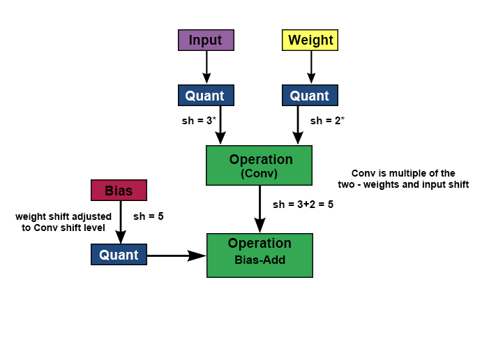
After Multiply-And-Accumulate function, the re-quantization step uses Scalar multipliers and shifts to avoid supporting division functions.
The quantization can be implemented per Tensor (per layer) or per output Channel (for Conv), if the dynamic range of each of the channel’s weights is quite different.
Methods of Quantization
Above all, Four methods of quantization listed in increasing order of accuracy,
- Without Vectors
- This post-training quantization flow determines the range of the activations without any vectors
- For INT8, the scaling factors are determined using the Scale / Shift values.
- Use Vectors to establish a range
- The vectors are used to know the range of activation.
- The activations are quantized based on the range determined by running vectors and registering the range of each Tensor
- Second pass Quantized Training
- After a model is completely trained, the model is retrained by inserting Quantization nodes to incrementally retrain for the error, etc.
- In this, the forward path uses quantized operations and the back-propagation is using floating-point arithmetic. (Tensorflow Lite – TFLite – Fake Quantization)
- Quantized Operator Flow (Q-Keras – Keras Quantization)
- There are new frameworks in development that perform quantization aware training (use quantized operands while training from the start)
For methods that do training, it requires that the customers provide their datasets and the definition for the loss/accuracy functions. It is likely that both are customer’s proprietary information that they would not readily share (a common scenario) and hence the need for the first two methods mentioned above.
Sample Results
The table below shows the results of quantization for some sample networks. The asymmetric UINT8 quantization, Per channel INT8, and UINT8 retrain quantization are compared with FP accuracy
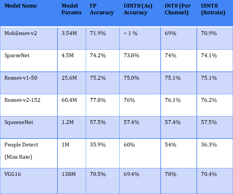
From the above result, some networks perform very poorly with standard quantization and may require per channel quantization and some would require retraining or other methods.
Moreover, retraining or training with quantized weights gives the best result but would require customers providing datasets, model parameters, Loss and accuracy functions, etc., which may be feasible for all the cases.
In Addition, some of the customer models have frozen (constant) weights and cannot re-train immediately after the release.
Methods to improve accuracy
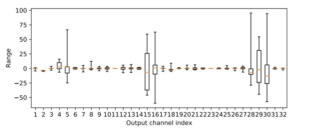
From the below figure, one of the main reasons for the loss of accuracy is the dynamic range of the weights across different channels
Dynamic Range
Methods to address the loss of accuracy without having to retrain are
- Per-channel
- Firstly, from the figure above, establishing a different scale for each of the output channels of a convolutional neural network (CNN) would preserve the accuracy as corroborated by the results
- Secondly, this introduces additional complexity to track the scaling of each channel and readjust the scaling value at the output activations to be at the same level to be used in the next layer
- Moreover, Hardware should track the per-channel scaling values and apply them on the output of each layer
- Reducing the Dynamic Range
- The distribution of the range of weights can be analyzed and weights that are anomalies, small in the count, and that is extreme can be clamped to the 2-Standard Deviation or 3-Standard Deviation.
- Usually, this step requires validation of the accuracies as some of the extreme weight may be required by the design
- Equalization
- The weights of each of the output layer are equalized in conjunction with the input weights of the next layers to normalize the ranges.
- Bias Correction
- Adjusts the bias values to compensate for the Quantization introduced bias error.
Quantization Impact on Frames / Sec
8-bit Quantization significantly improves the model performance by reducing the memory size and by doing 8-bit integer computations.
By adopting a dynamic bit of widths per layer, quantization gives even more performance benefits. Moreover, some layers can have quantization to 4-bit, 2-bit, and 1-bit quantization (ternary and binary neural networks) without significant loss of accuracy. These would be layer dependent and usually, the final layers tend to perform well with lower quantization granularity.
Binary and ternary operations are computationally less intensive than 8-bit Multiply Accumulates, yielding much lower power.
Even in cases where the hardware does not support 4-bit or 2-bit operations, the model compression achieved by just storing weights in a lesser number of bits reduces the storage and bus bandwidth requirement.
Gyrus Flows
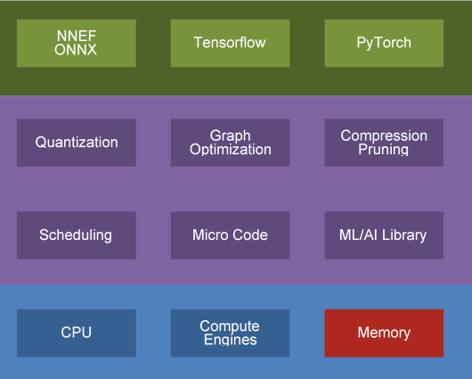
As a result, Gyrus developed several modules that bridge the gap between the Open Source AI Frameworks (Tensorflow, Pytorch, etc.) and the hardware from silicon vendors.,
The flows perform Graph Optimization, Compression, Pruning, Quantization, Scheduling, Compilation and ML/AI Library modules.
To learn more about our AI framework models, check out Gyrus AI Framework Modules
Specifically, in Quantization, the flows perform any of the three types of quantization (Power-2, Symmetric, and Asymmetric) and across the different methods of quantization (No Vectors, Vectors for Range, and Vectors for Retraining) mentioned above.
The flows also employ advanced methods to improve the quantization loss by doing per channel quantization, Dynamic range adjustment, and bias corrections. These flows are applicable for canned models or new models and the results presented by Gyrus quantization modules. Also, the quantization flows work in conjunction with compression and pruning and the quantization method used influences the compression scheme employed in the hardware.
Conclusion
Quantized fixed-point operations are the norm in edge computing. All Silicon vendors should support all or a sub-set of the different quantization schemes as there are advantages for each of them depending on the networks/models. To achieve close to FP accuracy, one needs to employ additional techniques than simple conversions. In addition, representing small bit widths for certain layers gives additional power and size advantages.
Types of Quantization
Power-2, Symmetric and Asymmetric quantization are the three types of quantization techniques of neural networks listed in increasing order of complexity and accuracy.
What is Symmetric Quantization
Symmetric quantization also sometimes referred to as linear quantization, which takes the maximum value in the tensor and equally divides the range using the maximum value. Here the activations will re-adjusted based on the input and output scaling factors.
What is Asymmetric Quantization
Asymmetric quantization fully utilizes the bits given but has a high complexity of implementation.
バックグラウンド
近年、深層学習ベースの機械学習(ML)モデルと人工知能(AI)モデルは、図1に示すように、帯域幅や遅延などのさまざまな要因でクラウドからエッジデバイスに移行しています。
消費電力、遅延、ハードウェアサイズは、エッジでの推論にとって重要な側面です。 さらに、GPUを使用してクラウドで開発されるモデルは浮動小数点モデルです。
最も重要なことは、ニューラルネットワークを実行するエッジ推論ハードウェアが、より低い電力とコストの予算に合わせて高価な浮動小数点ユニットをサポートする必要がないことが強く望まれていることです。 浮動小数点の対応するものと比較して、固定小数点の数学エンジンは非常に面積と電力効率が高いです。
さらに、クラウドで開発されたモデルは、精度を大幅に損なうことなく量子化する必要があります。 効率的な量子化メカニズムにより、32ビット浮動小数点(FP)モデルを8ビットINT演算に量子化できますが、ほとんどのモデルで精度が0.5%未満低下します。 このプロセスにより、メモリフットプリント、計算要件が削減され、モデルの推論を実行するために必要なレイテンシーと電力が削減されます。
GPU(FP演算を備えている)を含むほとんどのエッジデバイスは、現在、低精度で量子化された演算を利用しています。 一方、量子化はエッジ推論の事実上のステップです。 このブログでは、量子化を行うための一般的な方法、課題、およびそれらを克服する方法について説明しています。
量子化の種類
ニューラルネットワークには、複雑さと精度の高い順に、主に以下の3種類の量子化手法に分類があります。
- Power-2
- 対称
- 非対称
Power-2
Power-2量子化は、データの左右のシフトのみを使用して量子化を実行します。 バレルシフタはほとんどのハードウェアアーキテクチャの一部であるため、シフトの実装コストは非常に低くなります。 絶対最大値に基づいて最上位7ビット(INT8の場合)を維持するために、重みとバイアスは左または右にシフトすることによって量子化されます。 これらのビットは追跡され、操作の前後に必要に応じて再調整されます。
対称
複雑さの次のレベルは、線形量子化とも呼ばれる対称量子化です。これは、テンソルの最大値を取得し、最大値を使用して範囲を均等に分割します。 ここで、アクティベーションは、入力および出力のスケーリング係数に基づいて再調整されます。
非対称
最後に、非対称量子化は与えられたビットを完全に利用しますが、実装は非常に複雑です
Xf =スケール*(Xq – Xz)、ここでXfはXの浮動小数点値、Xqは量子化された値、Xzはゼロオフセットです。
ゼロオフセットは、ゼロ値が非小数値で表されるように調整されるため、ゼロパディングによってバイアス(Conv)が発生することはありません。
また。行列の乗算と畳み込みを実行する場合、すべてのオペランドごとに追加のAdd / Sub操作があり、多くのハードウェアアーキテクチャにはあまり役立ちません。
Conv = SUM((Xq-Xz)*(Wq-Wz))、ここでWは重み、Xは入力です。
ほとんどのレイヤーに存在するRELUなどの操作は負の値をノックオフするため、整数表現(INT8)は、UINT8表現と比較して、この表現では事実上少し失われます。
積和関数の後、再量子化ステップでは、スカラー乗数とシフトを使用して、除算関数のサポートを回避します。
各チャネルの重みのダイナミックレンジがまったく異なる場合、量子化はテンソルごと(レイヤーごと)または出力チャネルごと(変換の場合)に実装できます。
量子化の方法
とりわけ、精度の高い順に、4つの量子化方法があります。
- ベクトルなし
- このトレーニング後の量子化フローは、ベクトルなしでアクティベーションの範囲を決定します
- INT8の場合、倍率はスケール/シフト値を使用して決定されます。
- ベクトルを使用して範囲を確立する
- ベクトルは、活性化の範囲を知るために使用されます。
- アクティベーションは、ベクトルを実行し、各テンソルの範囲を登録することによって決定された範囲に基づいて量子化されます。
- 2番目のパスの量子化トレーニング
- モデルが完全にトレーニングされた後、量子化ノードを挿入してモデルを再トレーニングし、エラーなどを段階的に再トレーニングします。
- この場合、順方向パスは量子化された演算を使用し、逆方向伝搬は浮動小数点演算を使用します。 (Tensorflow Lite – TFLite –偽の量子化)
- 量子化された演算子フロー(Q-Keras – Keras量子化)
- 量子化対応トレーニングを実行する開発中の新しいフレームワークがあります。(最初からトレーニング中に量子化されたオペランドを使用します)
トレーニングを行う方法の場合、顧客がデータセットと損失/精度関数の定義を提供する必要があります。 どちらもお客様の専有情報であり、容易に共有できない可能性があり(一般的なシナリオ)、したがって、上記の最初の2つの方法が必要です。
サンプル結果
サンプルネットワークの量子化の結果を次の表に示します。 非対称UINT8量子化、チャネルごとのINT8、およびUINT8再トレーニング量子化が、FP精度と比較されています。
上記の結果から、一部のネットワークは標準の量子化では性能が非常に低く、チャネルごとの量子化が必要になる場合があり、一部のネットワークでは再トレーニングまたはその他の方法が必要になります。
さらに、量子化された重みを使用した再トレーニングまたはトレーニングは最良の結果をもたらしますが、データセット、モデルパラメータ、損失および精度関数などを提供する顧客が必要になります。 これはすべてのケースで当てはまります。
さらに、一部の顧客モデルは(一定の)ウェイトを凍結しており、リリース直後に再トレーニングできません。
精度を向上させる方法
下図から、精度が低下する主な理由の1つは、さまざまなチャネルにわたる重みのダイナミックレンジに起因することがわかります。
Dynamic Range
再トレーニングせずに精度の低下に対処する方法は次のとおりです。
- チャネルごと
- まず、上図から、畳み込みニューラルネットワーク(CNN)の出力チャネルごとに異なるスケールを確立すると、結果によって裏付けられる精度が維持されます。
- 次に、これにより、各チャネルのスケーリングを追跡し、出力アクティベーションでのスケーリング値を再調整して、次のレイヤーで使用するのと同じレベルにするための複雑さが増します。
- さらに、ハードウェアはチャネルごとのスケーリング値を追跡し、それらを各レイヤーの出力に適用する必要があります。
- ダイナミックレンジの縮小
- 重みの範囲の分布を分析し、異常でカウントが小さく、極端な重みを2標準偏差または3標準偏差に固定することができます。
- 通常、このステップでは、設計で極端な重量が必要になる場合があるため、精度の検証が必要です。
- イコライゼーション
- 各出力レイヤーの重みは、次のレイヤーの入力重みと組み合わせて均等化され、範囲が正規化されます。
- バイアス補正
- バイアス値を調整して、量子化によって導入されたバイアスエラーを補正します。
フレーム/秒に対する量子化の影響
8ビット量子化は、メモリサイズを削減し、8ビット整数計算を実行することにより、モデルの性能を大幅に向上させます。
レイヤーごとの幅の動的ビットを採用することにより、量子化はさらに多くの性能上の利点をもたらします。 さらに、一部のレイヤーでは、精度を大幅に損なうことなく、4ビット、2ビット、および1ビットの量子化(3値および2値ニューラルネットワーク)を使用できます。 これらはレイヤーに依存し、通常、最終レイヤーはより低い量子化粒度でうまく機能する傾向があります。
バイナリーとターナリ―演算は、8ビットの積和演算よりも計算量が少なく、電力がはるかに低くなります。
ハードウェアが、4ビットまたは2ビット操作をサポートしていない場合でも、より少ないビット数で重みを格納するだけでモデルの圧縮が実現されるため、ストレージとバスの帯域幅の要件が軽減されます。
Gyrusの開発フロー
その結果、Gyrusは、オープンソースAIフレームワーク(Tensorflow、 Pytorchなど)とシリコンベンダーのハードウェアの間のギャップを埋める複数のモジュールを開発しました。
フローは、グラフの最適化、圧縮、プルーニング、量子化、スケジューリング、コンパイル、およびML / AIライブラリモジュールを実行します。
AIフレームワークモデルの詳細については、Gyrus AIフレームワークモジュールをご覧ください。
具体的には、量子化では、フローは上記の3種類の量子化(Power-2、対称、非対称)のいずれかを実行し、上記のさまざまな量子化方法(ベクトルなし、範囲のベクトル、再トレーニングのベクトル)で実行します。
フローはまた、チャネルごとの量子化、ダイナミックレンジ調整、およびバイアス補正を行うことにより、量子化損失を改善するための高度な方法を採用しています。 これらのフローは、定型モデルまたは、新しいモデルおよび、Gyrus量子化モジュールによって提示される結果に適用できます。 また、量子化フローは、圧縮とプルーニングと連携して機能し、使用される量子化方法はハードウェアで採用されている圧縮スキームに影響を与えます。
結論
量子化された固定小数点演算は、エッジコンピューティングの標準です。 すべてのシリコンベンダーは、ネットワーク/モデルに応じてそれぞれに利点があるため、さまざまな量子化スキームのすべてまたはサブセットをサポートする必要があります。 FPに近い精度を実現するには、単純な変換以外の手法を採用する必要があります。 さらに、特定のレイヤーの小さなビット幅を表すと、パワーとサイズがさらに向上します。
量子化の種類
ニューラルネットワークには、R5その複雑さと精度により、昇順でリストされているPower-2、対称および非対称の3種類の量子化手法があります。
対称量子化とは
対称量子化は、線形量子化とも呼ばれます。これは、テンソルの最大値を取得し、最大値を使用して範囲を均等に分割します。 ここで、アクティベーションは、入力および出力の倍率に基づいて再調整されます。
非対称量子化とは
非対称量子化は、与えられたビットをすべて利用しますが、実装は非常に複雑です。

