Gyrus AI Blogs on New Ideas, Events, Updates for Video Anonymization, Streaming with AI/ML

Background

This blog outlines the steps involved and things to care about for transfer learning a propensity to buy model.

Sales team members could inundate with several prospects. The best use of their time is by lead scoring and focus on the prospects that have the best chance to close. hence, A Propensity To Buy model helps the sales team members to identify and focus on the deals that have a high probability to close.

However every business has its own process, dependencies, nuances etc.and a generic model cannot suit everyone. Certainly, this blog tries to outline the steps and the data to showcase the system for a custom Propensity To Buy model.

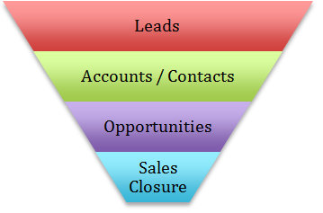
Typical steps in a sale are a gradual progression from Leads to Accounts to Opportunities to Sale Closure. Propensity models work best for the leads in the opportunity class as they have data from the interactions and also from the external factors.

Feature List

The relevant data to be pulled into the model as part of the customization are

• Product Categories
• $ Value of the product
• Dates, duration, the purpose of Sales Meetings
• Contacts, their titles/designations
• Technical and Business decision-makers
• Interaction with Contacts
• Time Progression from lead, to contact to an opportunity
• Current Probability to Close % as presented by the salesperson
• Past purchase history per customer
• Database Access with a snapshot of the sales data
• Social Media and Web Analytics from a campaign

There are additional features that can be accessed from the public domain

• Seasonality
• Customers Business (Earnings reports)
• Customer Business Activity (Press Releases)
• Customer Public Sentiment
• Social Media Activity
• Contact Specific Activity
• Competition Activity

These two feature-lists are not an exhaustive list, but however is a guideline to the type of parameters to use. The actual feature list could be smaller in cases where we do not have quality, snapshot data.

Data Cleanup and Normalization

As a first step, the input data is scrubbed for anomalies and data that is either not complete or visibly wrong (data entry related) is removed. There are tools for viewing and analyzing the datasets that can be used for this process. There are simple models that indicate the cases where the data is an anomaly and they can be included or discarded depending on the scenario.

All the features need to populate based on an instance of time. It is quite possible that some of the equivalent features are not available and a nominal value is in place. Some of the new models have the ability to take blank input value for some features, indicating that, that particular feature information is not available.

Usually, Data normalize, at two levels. Firstly, At a high level, you can check the data for mean, median and variance to be at the expected level. If it is not, the data normalize with a curve or an equation. Secondly, at the next level, the data is made to be within a range of [0-1] for all features. The third-party data as mention above are also subjects to clean up and normalization as well.

The data for each feature can be discrete values like a rating/ranking 1-5, or a number indicating price/cost or independent union.

The details of such data layer processing are here

Model Development

In general, the first batch of propensity models had a very small number of features implementing logistic regression, giving decent results. With the vast amount of information available, there is potential for much more learned decisions with more complex models.

Furthermore, there are two ways to re-train the model with custom dataset. The first method is to transfer learning. In this process, all the hyperparameters of the models retain and the learning process relearns the weights occur. Here then the weights can initialize to new values or can start from the previous weights. The decision depends on the convergence speed and accuracy.

If the first method does not converge to an acceptable accuracy level, the hyperparameters themselves will be changed. Here the intention is not to transfer from the previous learning experiment. Also, If the new dataset size is large enough to converge, all new data will be used for learning. However, if the dataset is not large enough, some of the generic previous dataset entries can be used.

Moreover, the models can be fine-tuned as new data is collected as well. Snapshots of the dataset can be made from the live data and processed as noted above. Also, one of the important factors in model revision control is to have the ability to go back to recreate the models, as data sets are changing. Using a data framework such as the one at Gyrus would help.

Above all, the usability of the explainability model and the bias check models in order to cross-check the results do not need to change much. However, the explainability model might need re-training with new data.

Results

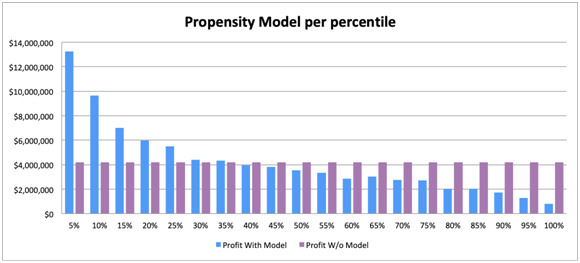
As a result, the below figure shows such exercise where the model saw a large upside in the net profit by focusing on the important accounts (up to 25 percentile). As can be seen from the chart, if there is an opportunity to approach, the result is similar to and without a model.

Conclusion

Gyrus has several similar models that can be referenced here.

Therefore, the propensity to buy is a very useful and productive model for real-life use-cases. also, it needs to tune/setup for the specific customer data to yield good results. Even more, in most cases of the box-model may not suit very well. Every model needs tools to efficiently do life cycle management and the corresponding explainability and bais check models.